How Changes in Economic Conditions Might Affect the Federal Budget: 2022 to 2032

Some of the uncertainty in budget projections stems from the fact that the federal budget is highly sensitive to economic conditions, which are difficult to accurately predict. If conditions differed from those in the Congressional Budget Office’s economic forecast, budgetary outcomes could diverge from those in the agency’s baseline budget projections.1

To show how variations in economic conditions might affect its budget projections, CBO analyzed how the budget might change if values of the following key economic variables differed from those in the agency’s forecast:

• The growth of productivity and, consequently, the growth of real gross domestic product (that is, GDP adjusted to remove the effects of inflation);
• Labor force growth, which would also affect real GDP growth;
• Interest rates; and
• Inflation and nominal interest rates (assuming that inflation-adjusted interest rates remain unchanged).

In those analyses, called the “rules of thumb,” CBO examined how slower productivity growth, slower labor force growth, higher interest rates, and higher inflation would increase deficits above the amounts in the agency’s baseline budget projections. However, the actual outcomes of any of those variables could be higher or lower than they are projected to be in CBO’s baseline. The rules of thumb are roughly symmetrical, so if productivity or the labor force increased more quickly than projected, or if interest rates or inflation were lower than projected, deficits would be smaller than they are in the agency’s baseline budget projections by about the same amounts.

Looking at deviations that would worsen budget deficits, CBO’s analysis yielded the following results:

• If productivity grew at a rate that was 0.1 percentage point slower each year than it does in the agency’s economic forecast, annual deficits would be larger than projected by amounts that would climb to $59 billion by 2032, CBO estimates. Over the 2023–2032 period, the cumulative deficit would be $292 billion larger than it is in CBO’s baseline projections.
• If the labor force grew at a rate that was 0.1 percentage point slower each year than the rate in CBO’s economic forecast and if the unemployment rate remained unchanged, annual deficits would be larger than those in the agency’s baseline budget projections by amounts that would grow each year and reach $27 billion by 2032, CBO estimates. The cumulative deficit for 2023 to 2032 would be $128 billion larger than it is in the agency’s baseline budget projections.
• If all interest rates—including both the rate on 3-month Treasury bills and the rate on 10-year Treasury notes—were 0.1 percentage point higher each year than they are in CBO’s economic forecast, deficits would increase progressively over the projection period by amounts that would rise to $41 billion in 2032, if other variables were held constant. The cumulative deficit for 2023 to 2032 would be $285 billion larger than it is in the agency’s baseline projections.
• If all wage and price indexes—including the GDP price index, the consumer price index for all urban consumers (CPI-U), the chained CPI-U, and the employment cost index for wages and salaries of workers in private industry—grew at a rate that was 0.1 percentage point faster each year than the rate in CBO’s economic forecast, annual deficits would be larger than projected by amounts that would climb to $43 billion by 2032. That total reflects the effects of higher nominal GDP and taxable income resulting from increased inflation, as well as higher nominal interest rates to keep real interest rates unchanged. The cumulative deficit for the 2023–2032 period would be $262 billion larger than projected.

Background

When economic conditions differ from those in the agency’s forecast, actual federal spending and revenues are likely to differ from CBO’s projections because economic conditions affect federal revenues and outlays in several ways. Revenues depend on the total amount of income that is subject to taxation, including wages and salaries, other income received by individuals, and corporate profits. Those types of income generally rise or fall (though not necessarily proportionally) in response to changes in economic growth and inflation. In addition, the Treasury regularly refinances portions of the government’s outstanding debt—and issues more debt to finance new deficits—at market interest rates. Thus, the amount that the federal government spends to pay interest on its debt is directly tied to those rates. Spending for many mandatory programs is also affected by economic growth and inflation—either explicitly (for example, through cost-of-living adjustments) or indirectly (for example, through the number of beneficiaries). Finally, although actual spending for discretionary programs is determined by lawmakers, CBO’s projections of such spending are affected by changes in inflation.2

Economic conditions are uncertain and difficult to predict and, therefore, could differ from those in CBO’s forecast for a variety of reasons. For example, inflation has been much higher and more persistent than CBO and other forecasters had anticipated last year.3 Future changes in policy can also cause economic outcomes to differ from CBO’s projections. One of many examples is that future changes in immigration policy could significantly affect the growth of the labor force. Furthermore, for policy changes that are already set in law and reflected in the baseline, the economic effects are subject to considerable uncertainty, and the actual effects of such changes may diverge from CBO’s projections. Finally, sometimes changes in economic conditions, such as turning points in the business cycle, cannot be accurately predicted from available information.

The Economic Variables That CBO Examined

To develop the rules of thumb for changes in the four key economic variables, CBO estimated how differences in each of those variables would affect the budget projections. For each analysis, the values of the economic variables differ from those in the agency’s forecast by 0.1 percentage point each year starting in January 2022.4 In the first two analyses—slower productivity growth and slower labor force growth—real GDP growth is slower, thereby also affecting many other variables that affect the budget more directly, such as wages and salaries and interest rates. In the third and fourth analyses—higher interest rates and higher inflation—real GDP growth remains unchanged by design, but other variables such as interest payments on federal debt are affected. CBO has produced an interactive workbook in which users can create their own alternative scenarios for the key variables to see how revenues, outlays, deficits, and debt might differ from the agency’s baseline budget projections.5

For simplicity, CBO constructed the scenarios so that the variables targeted in the four rules of thumb differ from those in the agency’s forecast by 0.1 percentage point in the direction that would worsen budget deficits. The scenarios are not intended to indicate how actual economic conditions might differ from those in CBO’s projections; differences in either direction should be equally likely. The agency estimates that there is roughly a two-thirds chance that the average annual growth rate of real GDP over the next five years will be within 1.3 percentage points above or below the projected rate. Similarly, there is about a two-thirds chance that the average annual rate of inflation (as measured by the GDP price index) over the next five years will be within 1.2 percentage points of the rate in CBO’s forecast in either direction, and the probability is the same that the average interest rate (on 10-year Treasury notes, in real terms) will be within 1.1 percentage points of the forecast rate in either direction.6

Productivity Growth. In this scenario, productivity growth is 0.1 percentage point slower each year than it is in CBO’s economic forecast, causing real GDP to be 1.2 percent lower in 2032 than forecast (see Table 1). Slower productivity growth, in turn, would affect other economic variables, such as wage rates and interest rates.

Labor Force Growth. In the second scenario, the labor force’s rate of growth is 0.1 percentage point slower each year than the rate in the agency’s economic forecast, causing real GDP to be 0.7 percent lower than forecast in 2032. If the population grew at the rate that CBO projects, the slower growth of the labor force would cause the labor force participation rate to fall below the agency’s current estimates. That difference would grow by a roughly equal amount each year until the labor force participation rate was 0.7 percentage points lower in 2032 than forecast. Like slower productivity growth, slower labor force growth would affect other economic variables.

Interest Rates. In the third scenario, interest rates are 0.1 percentage point higher each year than those in CBO’s forecast. Inflation is held equal to the forecast rate in this scenario, so the corresponding rule of thumb shows the effects of higher real interest rates. Unlike the other scenarios, this scenario does not include any changes to the projected amounts of interest payments made or received by individuals or businesses.

Inflation. In the fourth scenario, inflation and interest rates are 0.1 percentage point higher each year than they are in the agency’s economic forecast. All economic indicators that are measured as nominal values, such as GDP and taxable income, increase in response to higher inflation, and all interest rates are 0.1 percentage point higher than they are in the economic forecast, as in the third scenario. Indicators that are measured as real values, such as real GDP and real interest rates, are the same as they are in CBO’s economic forecast.

Applying the Rules of Thumb

CBO’s rules of thumb provide a rough sense of how changes in those economic variables would affect the federal government’s revenues and outlays if current laws remained generally unchanged.7 The rules of thumb are roughly symmetrical and scalable, which means that they can be used to analyze scenarios in which values for those variables differ from the ones presented here, with some caveats.

Symmetry. Each rule of thumb is roughly symmetrical. Thus, if the growth of productivity or the labor force was 0.1 percentage point faster than in CBO’s baseline or if interest rates or inflation were 0.1 percentage point lower than in CBO’s baseline, the effects would be about the same as those shown here, but with the opposite sign.

Scalability. In addition to being symmetrical, the rules of thumb are roughly scalable—that is, an increase or decrease in the value of a given economic variable will produce a roughly proportional increase or decrease in the resulting budgetary effects. For example, if productivity growth was 0.2 percentage points slower each year than it is in CBO’s economic forecast rather than 0.1 percentage point slower as it is in the scenario discussed here, the annual increase in the deficit would be roughly double.

However, the scalability of the rules of thumb is limited. The more the values of economic variables differ from those in CBO’s forecast, the less accurate the estimates produced using the rules of thumb are likely to be. Although the productivity and labor force scenarios incorporate a broad set of interactions among several economic variables, all four rules of thumb are nevertheless simplified and do not account for more complex interactions among variables—such as those among growth in real GDP, inflation, and the unemployment rate. That limitation becomes more pertinent as the difference between the value of an economic variable in a given scenario and in CBO’s forecast increases. Certain elements of the tax code and some provisions relating to mandatory outlays also make it likely that, as such differences increase, estimates produced using the rules of thumb become less accurate.

Moreover, the rules of thumb are based on scenarios in which the values of variables differ from the values in CBO’s economic forecast by the same amount each year. The rules of thumb can be applied to scenarios in which the differences vary somewhat from year to year, but they cannot be used to accurately estimate the budgetary effects of significant variations in those differences over the 2022–2032 period. For example, if the rate of labor force growth differed from the value in CBO’s forecast by 0.5 percentage points in 2032 but was the same as the forecast value in all other years, the average annual difference would be a little less than 5 basis points (that is, 0.05 percentage points).8 But CBO’s estimate of the budgetary effect over the same period would not be one-half the amount shown for the scenario for slower labor force growth (a difference of 0.1 percentage point each year), nor would the agency’s estimate of the budgetary effect in 2032 be five times greater than the value for that year under the illustrative scenario. Both estimates would be considerably smaller than those ratios.

To assess the scalability of the rules of thumb, CBO compared estimates produced from the simplified calculations in its online workbook with estimates made from a broader set of models that the agency uses to assess the effects of economic changes on the budget. CBO found that the four rules of thumb produced approximations of the estimates generated by CBO’s economic and budget models as long as the values for each of the variables did not differ from the forecast values by more than a certain amount. Specifically, the rules of thumb were scalable as long as the annual differences from the forecast values were within the following ranges:

• For productivity growth, between −0.5 percentage points and 0.5 percentage points;
• For labor force growth, between −0.75 percentage points and 0.75 percentage points;
• For interest rates, between −1.0 percentage point and 1.0 percentage point; and
• For inflation, between −1.0 percentage point and 1.0 percentage point.

In general, differences outside those ranges in any given year would generate budgetary effects that could not be reasonably approximated by the rules of thumb and therefore would require a more detailed analysis.

Caveats. If economic conditions changed in such a way that they reflected the changes incorporated in two or more of the simplified scenarios, the budgetary effects would most likely differ from the sum of the estimates calculated with the individual rules of thumb. For example, if rates of productivity growth and labor force growth were both slower than they are in CBO’s economic forecast, the two effects would interact and possibly lower output growth by more or less than would be suggested by simply adding those effects.

The rules of thumb capture the budgetary effects of specified changes in the economy, but they do not account for the source of those changes, which could include changes in policy. For example, a proposal might call for an increase in government spending that would affect inflation. The rule of thumb for inflation approximates the budgetary effects that would result from the estimated changes in inflation—but it does not incorporate the budgetary effects of the increased spending itself, nor does it encompass other effects on the economy besides a change in inflation.

In addition, some changes in policy could alter how changes in the economy affect the federal budget. For example, a new tax policy that changed effective tax rates would probably affect the relationship between changes in the economy and revenues. Changes to that relationship would cause the budgetary effects resulting from changes in the economy to differ from those that would be estimated using the rules of thumb.

Changes in Productivity Growth and Labor Force Growth

The growth of productivity and the growth of the labor force are important determinants of real GDP growth. Faster productivity growth and faster labor force growth both lead to greater economic growth and thus reduce budget deficits. Slower productivity growth and slower labor force growth both reduce the growth of GDP, thereby worsening budget deficits.9

Slower Productivity Growth

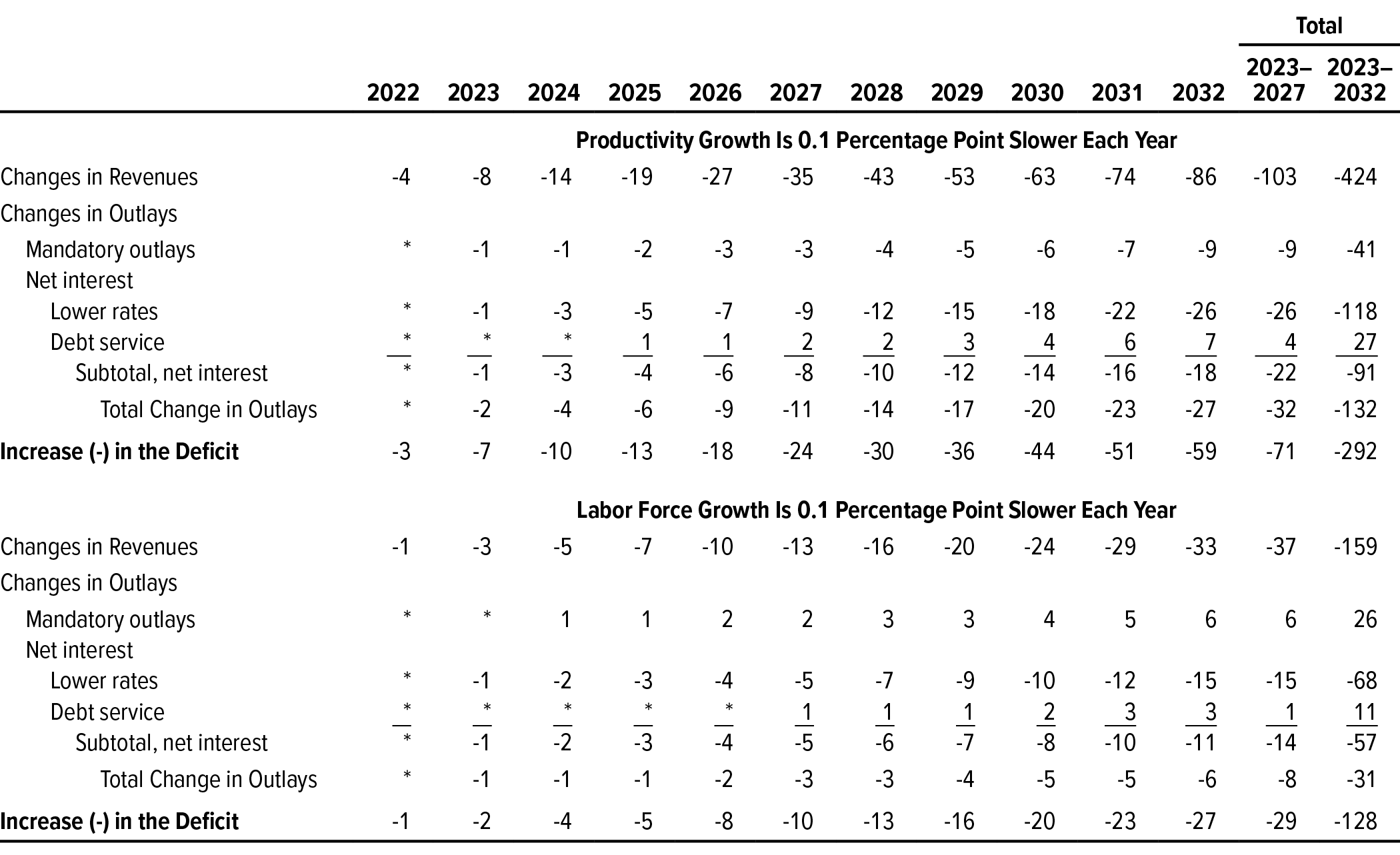
The first rule of thumb illustrates the budgetary effects of productivity growth that is slightly weaker than CBO currently anticipates. Specifically, if productivity grew at a rate that was 0.1 percentage point slower each year than the rate in the agency’s economic forecast, annual deficits would be larger than projected by amounts that would climb to $59 billion by 2032, CBO estimates. In the 2023–2032 period, the cumulative deficit would be $292 billion larger than it is in CBO’s baseline projections (see Table 2).

In this analysis, CBO examined how the slower growth of productivity might affect GDP, income, and interest rates.10 The agency found that slower-than-anticipated productivity growth would lead to slower growth in GDP because both labor and capital would be producing less per unit than projected in CBO’s current economic forecast. If workers produced less, the average hourly wage rate would be lower; therefore, the supply of labor would also initially decline but would recover back to the agency’s baseline in later years. As a result, total labor income would be lower. Meanwhile, if capital produced less output, the returns on that capital would also decline, further decreasing total taxable income. Lower returns on capital would also cause private investment to be lower. Treasury securities compete with other investments for investors’ money, so those lower rates of return on private investments imply that rates on Treasury securities would also be lower. Other variables, such as the unemployment rate and inflation, could be affected as well; however, this simplified scenario does not include the effects of changes in those variables.

If actual productivity growth was 0.1 percentage point slower each year than it is projected to be, GDP and total income would be about 1.2 percent lower by 2032 than they are in the current forecast, CBO estimates. Meanwhile, interest rates in 2022 would be about 1 basis point below those in the agency’s forecast, and that difference would increase by roughly 1 additional basis point in each subsequent year. By 2032, interest rates would be about 9 basis points lower than in the forecast (see Table 1).

Effects on Tax Revenues. If economic growth slowed in each year as a result of lower productivity growth, taxable income would also grow more slowly than projected, and tax revenues would fall below CBO’s baseline projections by increasing amounts over time, resulting in a shortfall of $86 billion in 2032. Between 2023 and 2032, the drop in revenues stemming from the slower growth in income would increase deficits by a total of $424 billion.

Effects on Mandatory Spending. Over the 2023–2032 period, slower income growth would also lead to a $41 billion net decrease in mandatory outlays for programs whose spending is either explicitly or implicitly linked to wage growth. Outlays for Medicare, Medicaid, unemployment insurance, and Social Security would decrease by $47 billion; that decrease would be partially offset by an increase of $7 billion in outlays for the refundable portions of the earned income tax credit, the child tax credit, and the American Opportunity Tax Credit.11

Effects on Net Interest Costs. Because slower productivity growth would push interest rates down, the amount of interest that the federal government would pay on the debt projected in CBO’s baseline between 2023 and 2032 would decrease by $118 billion. However, if revenues were reduced by the amounts indicated above, the federal government would need to borrow more than projected to finance the resulting net increase in the deficit. That additional borrowing would add $27 billion to interest payments between 2023 and 2032. Together, those effects would result in net interest outlays that were $91 billion less than the amount in the agency’s baseline projections over the 2023–2032 period.12

Slower Labor Force Growth

The second rule of thumb illustrates the budgetary effects of the labor force’s growing more slowly than CBO anticipates. Specifically, if annual growth in the labor force was 0.1 percentage point slower than it is in CBO’s economic forecast and the unemployment rate remained unchanged, annual deficits would be larger than those in the agency’s baseline budget projections by amounts that would grow each year and reach $27 billion by 2032, CBO estimates. The cumulative deficit for 2023 to 2032 would be $128 billion larger than it is in the agency’s baseline budget projections (see Table 2). The budgetary effects under this scenario are considerably smaller than those under the scenario involving slower productivity growth because the resulting economic effects are smaller (see Table 1).

To arrive at this rule of thumb, CBO began by analyzing how the slower growth of the labor force under the illustrative scenario might affect GDP, income, and interest rates. Slower-than-projected growth in the labor force would push the average wage rate above CBO’s current estimate. Those higher wage rates would initially bring about a small boost in labor income and in the supply of labor, which would partially offset the effects of the initial decline in labor force growth. Despite those effects, total labor income would be less than it is in CBO’s baseline. Meanwhile, the number of workers using a given amount of capital would fall below the number projected in CBO’s economic forecast, so the returns on that capital would decline as well. As described above, the resulting decline in the rates of return on private investment would imply that interest rates on Treasury securities would be lower than they are in CBO’s economic forecast. Although other variables—including the unemployment rate, inflation, the distribution of labor income, and rates of retirement—could also be affected by the labor force’s growing more slowly than projected, this rule of thumb does not reflect the effects of such changes.

In CBO’s estimation, if the rate of growth in the labor force was 0.1 percentage point slower than anticipated, GDP growth would also be slower each year. Meanwhile, interest rates in 2022 would be slightly lower than forecast, and that difference would increase in each subsequent year. By 2032, GDP and labor income would be 0.7 percent lower than they are in CBO’s forecast, and interest rates would be about 5 basis points lower (see Table 1).

Effects on Tax Revenues. The slower economic growth would cause taxable labor income and profits to grow more slowly than projected, resulting in tax revenues that were less than the amounts in CBO’s baseline projections. The shortfall would increase over time, reaching $33 billion in 2032 and totaling $159 billion over the 2023–2032 period.

Effects on Mandatory Spending. The higher-than-projected wage rates and the smaller-than-projected number of workers would, on net, add a total of $26 billion to mandatory outlays between 2023 and 2032. Specifically, because outlays for Medicare, Medicaid, and Social Security are linked to wage growth, mandatory spending for those programs would increase by $35 billion. But because there would be fewer workers and higher wages, $10 billion of that amount would be offset by a decrease in outlays for unemployment insurance benefits and the refundable portions of the earned income tax credit, the child tax credit, and the American Opportunity Tax Credit.

Effects on Net Interest Costs. Between 2023 and 2032, the lower interest rates that resulted from the slower growth of the labor force would reduce the amount of interest that the federal government would pay on the debt projected in CBO’s baseline by about $68 billion. However, the reduction in revenues and slight increase in mandatory spending would increase the deficit, requiring the federal government to borrow more than projected. That additional borrowing would add $11 billion to interest payments. Overall, CBO estimates that net interest outlays between 2023 and 2032 would be $57 billion less than they are in the agency’s baseline projections.

Changes in Interest Rates and Inflation

Changes in interest rates and inflation affect the federal budget. All else being equal, higher interest rates would increase the flow of interest payments to and from the federal government. Higher inflation and interest rates would raise both revenues and outlays, though the effect on outlays would be larger. Lower interest rates and inflation would have the opposite effects.

Higher Interest Rates

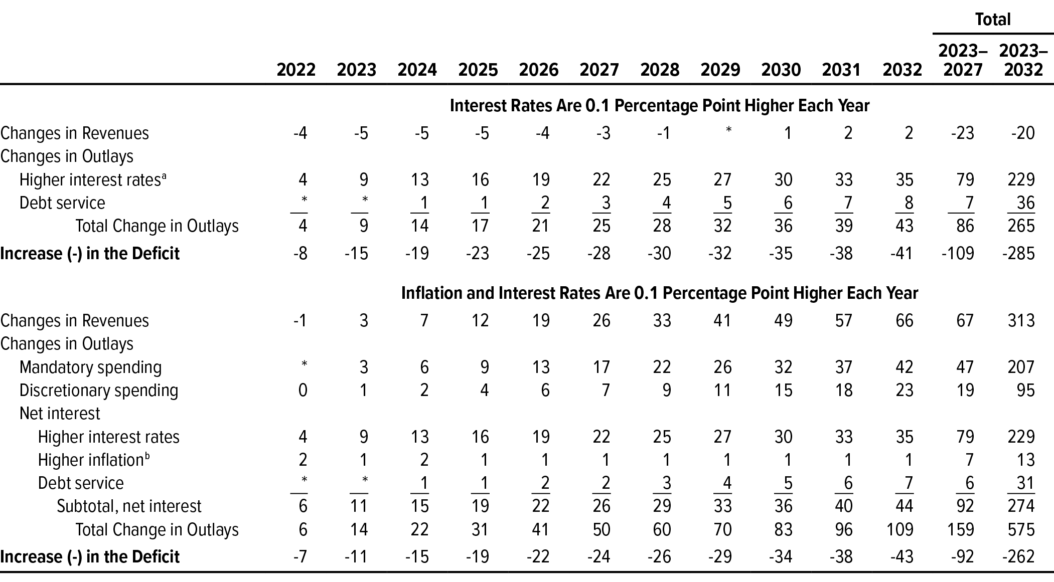
The third rule of thumb illustrates the budget’s sensitivity to an increase in interest rates when all other economic variables are left unchanged. In the illustrative scenario, all interest rates—including both the rate on 3-month Treasury bills and the rate on 10-year Treasury notes—are 0.1 percentage point higher each year than they are in CBO’s economic forecast. Under that scenario, in CBO’s estimation, deficits would exceed those in CBO’s baseline projections by amounts that would rise to $41 billion in 2032. The cumulative deficit for 2023 to 2032 would be $285 billion larger than it is in the agency’s baseline projections (see Table 3).

Effects on Interest Costs. Most of the increase in deficits resulting from higher interest rates would arise because the government’s costs of borrowing would be larger. As the Treasury replaced maturing securities and increased its borrowing to cover future deficits, the budgetary effects of higher interest rates would mount. Under this scenario, the added costs of higher interest rates on the debt projected in CBO’s baseline would reach $35 billion in 2032 and would total $229 billion for the 2023–2032 period, after accounting for a small increase in additional interest payments received by the government.13

The larger deficits generated by an increase in interest rates would require the Treasury to borrow more than it is projected to borrow in CBO’s baseline. That additional borrowing would raise the cost of servicing the debt by amounts that would increase each year and reach $8 billion in 2032. Between 2023 and 2032, the additional borrowing would add a total of $36 billion to the cost of servicing the federal debt.

Effects on Revenues. As part of conducting monetary policy, the Federal Reserve buys and sells Treasury and other securities. The Federal Reserve also pays interest on reserves (deposits that banks hold at the central bank). The interest that the Federal Reserve earns on its portfolio of securities and the interest that it pays on reserves affect its remittances to the Treasury, which are counted as revenues. If all interest rates were 0.1 percentage point higher than CBO projects, the Federal Reserve’s remittances over the next few years would be smaller than projected because higher interest payments on reserves would outstrip the additional earnings from interest on its portfolio. Over time, however, the current holdings in the portfolio would mature and be replaced with higher-yielding investments; as a result, by 2030, the Federal Reserve’s remittances would be larger. Overall, rates that were 0.1 percentage point higher than those in CBO’s economic forecast would (all else being equal) cause revenues from the Federal Reserve’s remittances over the 2023–2032 period to be $20 billion less than projected.

Higher Inflation

The fourth rule of thumb shows the budgetary effects of inflation that is 0.1 percentage point higher each year than it is in CBO’s baseline. All economic variables that are measured as nominal values, such as GDP, taxable income, and wage rates, increase by the same percentage in response to higher inflation. As a result, those that are measured as real values, such as real GDP and real interest rates, remain unchanged. In this scenario, all wage and price indexes grow 0.1 percentage point faster each year than they do in CBO’s economic forecast, and all interest rates are 0.1 percentage point higher each year, as they are in the third rule of thumb. As a result, higher inflation would increase both revenues and outlays, although the effect on outlays would be greater, resulting in larger budget deficits, on net.

Under this scenario, total revenues between 2023 and 2032 would be $313 billion more than they are in the agency’s baseline budget projections, and total outlays would be $575 billion more, CBO estimates. The cumulative deficit for the 2023–2032 period would be $262 billion larger than projected (see Table 3).

Effects on Revenues. Larger increases in prices and wage rates generally lead to greater labor income, profits, and other income, which in turn generate larger collections of individual income taxes, payroll taxes, and corporate income taxes. Many provisions in the individual income tax system—including the income thresholds for the tax brackets—are adjusted, or indexed, for inflation. Therefore, the share of taxpayers’ income that is taxed at certain rates does not change very much when income increases because of higher inflation, so tax collections tend to rise roughly proportionally with income under those circumstances. However, not all parameters of the individual income tax system are indexed for inflation. For example, the income thresholds for the surtax on investment income are fixed in nominal dollars, so if income rose because of inflation, the surtax would apply to a larger share of taxpayers’ income.

For the payroll tax, rates are mostly the same for all income levels, and the maximum amount of earnings subject to the Social Security tax rises (after a lag) with average wages in the economy. Higher nominal wages therefore lead to a roughly proportional increase in payroll tax revenues. Similarly, nearly all corporate profits are taxed at a single statutory rate of 21 percent. Consequently, an increase in profits resulting from higher inflation generates a roughly proportional increase in corporate tax revenues. Finally, higher nominal interest rates would first reduce and then increase revenues from the Federal Reserve’s remittances to the Treasury. All told, inflation that was 0.1 percentage point higher than forecast each year would add $313 billion in revenues to the amounts in the agency’s baseline budget projections between 2023 and 2032.

Effects on Mandatory Spending. Higher inflation would also increase the cost of a number of mandatory spending programs, adding $207 billion to projected spending, CBO estimates. Benefits for many mandatory programs are automatically adjusted each year to reflect increases in prices. Specifically, benefits paid for Social Security, federal employees’ retirement programs, disability compensation for veterans, the Supplemental Nutrition Assistance Program, Supplemental Security Income, child nutrition programs, and the refundable portion of the earned income tax credit, among others, are adjusted (after a lag) for changes in the consumer price index, one of its components, or another measure of inflation. Many of Medicare’s payment rates are also adjusted annually for inflation. Spending for some other programs, such as Medicaid, is not formally indexed to changes in prices but nevertheless tends to grow with inflation because the costs of providing benefits under those programs increase as nominal wages and prices rise. In addition, to the extent that benefit payments in retirement and disability programs are linked to participants’ preenrollment wages, increases in nominal wages resulting from higher inflation would boost future outlays for those programs.

Effects on Discretionary Spending. CBO’s baseline projections reflect the assumption that discretionary funding—including obligation limitations on certain transportation programs—will increase with inflation (as measured by a weighted average of the GDP price index and wages and salaries for workers in private industry) from the amounts currently provided. For most discretionary programs, inflation that was 0.1 percentage point higher each year than the rates underlying CBO’s economic forecast would boost projected funding (and therefore outlays) each year over the 2023–2032 period. Some appropriations—mostly those made by the Infrastructure Investment and Jobs Act—are made for years beyond the current year. Inflation that was higher than what is projected in CBO’s economic forecast would not change that specified funding but would affect funding projected for the years following those advance appropriations.14 In total, inflation that was 0.1 percentage point higher each year than the rates underlying CBO’s economic forecast would increase discretionary outlays in CBO’s baseline over the 2023–2032 period by a total of $95 billion.

Effects on Net Interest Costs. Inflation also has an effect on net outlays for interest, primarily because all interest rates would be 0.1 percentage point higher each year. Higher inflation also increase the cost to the government of inflation-indexed securities.15 The direct effect of such higher interest rates and inflation would be to add $242 billion in interest costs to CBO’s baseline projections of outlays. Moreover, the effects of higher inflation would increase federal debt, boosting interest costs by an additional $31 billion between 2023 and 2032.

---